Optimization Using Hopfield Network and Associate Memory Network

 

Optimization is an action of making something such as design, situation, resource, and system as effective as possible. Using a resemblance between the cost function and energy function, we can use highly interconnected neurons to solve optimization problems. Such a kind of neural network is Hopfield network, that consists of a single layer containing one or more fully connected recurrent neurons. This can be used for optimization.

Points to remember while using Hopfield network for optimization −

• The energy function must be minimum of the network.

• It will find satisfactory solution rather than select one out of the stored patterns.

• The quality of the solution found by Hopfield network depends significantly on the initial state of the network.

Travelling Salesman Problem

Finding the shortest route travelled by the salesman is one of the computational problems, which can be optimized by using Hopfield neural network.

Basic Concept of TSP

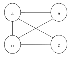
Travelling Salesman Problem TSP

is a classical optimization problem in which a salesman has to travel n cities, which are connected with each other, keeping the cost as well as the distance travelled minimum. For example, the salesman has to travel a set of 4 cities A, B, C, D and the goal is to find the shortest circular tour, A-B-C–D, so as to minimize the cost, which also includes the cost of travelling from the last city D to the first city A.

Matrix Representation

Actually each tour of n-city TSP can be expressed as n × n matrix whose i_th row describes the i_th city’s location. This matrix, M, for 4 cities A, B, C, D can be expressed as follows −

M=⎡⎣⎢⎢⎢A:B:C:D:1000010000100001⎤⎦⎥⎥⎥

Solution by Hopfield Network

While considering the solution of this TSP by Hopfield network, every node in the network corresponds to one element in the matrix.

Energy Function Calculation

To be the optimized solution, the energy function must be minimum. On the basis of the following constraints, we can calculate the energy function as follows −

Constraint-I

First constraint, on the basis of which we will calculate energy function, is that one element must be equal to 1 in each row of matrix M and other elements in each row must equal to 0 because each city can occur in only one position in the TSP tour. This constraint can mathematically be written as follows −

∑j=1nMx,j=1forx∈{1,...,n}

Now the energy function to be minimized, based on the above constraint, will contain a term proportional to −

∑x=1n(1−∑j=1nMx,j)2

Constraint-II

As we know, in TSP one city can occur in any position in the tour hence in each column of matrix M, one element must equal to 1 and other elements must be equal to 0. This constraint can mathematically be written as follows −

∑x=1nMx,j=1forj∈{1,...,n}

Now the energy function to be minimized, based on the above constraint, will contain a term proportional to −

∑j=1n(1−∑x=1nMx,j)2

Cost Function Calculation

Let’s suppose a square matrix of (n × n) denoted by C denotes the cost matrix of TSP for n cities where n > 0. Following are some parameters while calculating the cost function −

• C_{x, y} − The element of cost matrix denotes the cost of travelling from city x to y.

• Adjacency of the elements of A and B can be shown by the following relation −

Mx,i=1andMy,i±1=1

As we know, in Matrix the output value of each node can be either 0 or 1, hence for every pair of cities A, B we can add the following terms to the energy function −

∑i=1nCx,yMx,i(My,i+1+My,i−1)

On the basis of the above cost function and constraint value, the final energy function E can be given as follows −

E=12∑i=1n∑x∑y≠xCx,yMx,i(My,i+1+My,i−1)+

[γ1∑x(1−∑iMx,i)2+γ2∑i(1−∑xMx,i)2]

Here, γ₁ and γ₂ are two weighing constants.

 

 

Associate Memory Network

These kinds of neural networks work on the basis of pattern association, which means they can store different patterns and at the time of giving an output they can produce one of the stored patterns by matching them with the given input pattern. These types of memories are also called Content-Addressable Memory CAM

. Associative memory makes a parallel search with the stored patterns as data files.

Following are the two types of associative memories we can observe −

• Auto Associative Memory
• Hetero Associative memory

Auto Associative Memory

This is a single layer neural network in which the input training vector and the output target vectors are the same. The weights are determined so that the network stores a set of patterns.

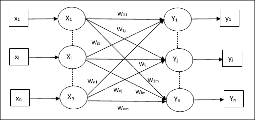
Architecture

As shown in the following figure, the architecture of Auto Associative memory network has ‘n’ number of input training vectors and similar ‘n’ number of output target vectors.

Training Algorithm

For training, this network is using the Hebb or Delta learning rule.

Step 1 − Initialize all the weights to zero as w_ij = 0 i=1ton,j=1ton

Step 2 − Perform steps 3-4 for each input vector.

Step 3 − Activate each input unit as follows −

xi=si(i=1ton)

Step 4 − Activate each output unit as follows −

yj=sj(j=1ton)

Step 5 − Adjust the weights as follows −

wij(new)=wij(old)+xiyj

Testing Algorithm

Step 1 − Set the weights obtained during training for Hebb’s rule.

Step 2 − Perform steps 3-5 for each input vector.

Step 3 − Set the activation of the input units equal to that of the input vector.

Step 4 − Calculate the net input to each output unit j = 1 to n

yinj=∑i=1nxiwij

Step 5 − Apply the following activation function to calculate the output

yj=f(yinj)={+1−1ifyinj>0ifyinj⩽0

Hetero Associative memory

Similar to Auto Associative Memory network, this is also a single layer neural network. However, in this network the input training vector and the output target vectors are not the same. The weights are determined so that the network stores a set of patterns. Hetero associative network is static in nature, hence, there would be no non-linear and delay operations.

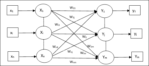
Architecture

As shown in the following figure, the architecture of Hetero Associative Memory network has ‘n’ number of input training vectors and ‘m’ number of output target vectors.

Training Algorithm

For training, this network is using the Hebb or Delta learning rule.

Step 1 − Initialize all the weights to zero as w_ij = 0 i=1ton,j=1tom

Step 2 − Perform steps 3-4 for each input vector.

Step 3 − Activate each input unit as follows −

xi=si(i=1ton)

Step 4 − Activate each output unit as follows −

yj=sj(j=1tom)

Step 5 − Adjust the weights as follows −

wij(new)=wij(old)+xiyj

Testing Algorithm

Step 1 − Set the weights obtained during training for Hebb’s rule.

Step 2 − Perform steps 3-5 for each input vector.

Step 3 − Set the activation of the input units equal to that of the input vector.

Step 4 − Calculate the net input to each output unit j = 1 to m;

yinj=∑i=1nxiwij

Step 5 − Apply the following activation function to calculate the output

yj=f(yinj)=⎧⎩⎨⎪⎪+10−1ifyinj>0ifyinj=0ifyinj<0